Chapter 2 Sums
2.1 Notation
The summation of an explicit sequence denoted as a succession of summations like $a_1+a_2+\cdots+a_n$ can be written in the delimited form $\sum_{k=1}^na_k$. Here, $a_k$ is called the summand, and $k$ is an index variable said to be bound to the summation. Summations can also be written in the general form like $\sum_{1\leq k\leq n}a_k$, making it easier for manipulations such as substitution of index variables.
2.2 Sums and Recurrences
There’s a neat relation between sums and recurrences. A sum like
$$S_n=\sum_{k=0}^na_k$$
is equivalent to the recurrence
$$\begin{aligned}S_0&=a_0;\\S_n&=S_{n-1}+a_n,\quad\text{for $n>0$.}\end{aligned}$$
Therefore we can evaluate a sum using methods of solving recurrences, such as the repertoire method we’ve learnt in Chapter 1.
We developed a technique that can reduce any recurrence of the form
$$a_nT_n=b_nT_{n-1}+c_n$$
to a sum, by multiplying both sides by a summation factor $s_n$, such that $s_nb_n=s_{b-1}a_{n-1}$. Then we can view $s_na_nT_n$ as a whole and go on.
2.3 Manipulation of Sums
To evaluate sums in closed form or to simplify sums, the key to success is the ability to change one summation into another under a few rules.
Let $K$ be any finite set of integers. Sums over the elements of $K$ can be transformed by using these three rules:
$$\begin{aligned}\sum_{k\in K}{ca_k}&=c\sum_{k\in K}{a_k};&&\text{(distributive law)}\\\sum_{k\in K}(a_k+b_k)&=\sum_{k\in K}a_k+\sum_{k\in K}b_k;&&\text{(associative law)}\\\sum_{k\in K}a_k&=\sum_{p(k)\in K}a_{p(k)}.&&\text{(commutative law)}\end{aligned}$$
The commutative law allows us to reorder terms. Here $p(k)$ is any permutation of the set of all integers. Actually, it’s a special case of a more generalized rule:
Suppose there’s an arbitrary function $f:J\to K$ that takes an integer $j\in J$ into an integer $k\in K$. The formula is
$$\sum_{j\in J}a_{f(j)}=\sum_{k\in K}a_k\#f^-(k),$$
where $\#f^-(k)$ stands for the number of elements in the set $f^-(k)=\big\{j\mid f(j)=k\big\}$.
If $f$ is an one-to-one correspondence between $J$ and $K$, we have $\#f^-(k)=1$ for all $k$, and the formula reduces to the commutative law.
2.4 Multiple Sums
Multiple sums follow two additional rules:
$$\begin{aligned}\sum_{P(j,k)}a_{j,k}&=\sum_j\sum_ka_{j,k}\big[P(j,k)\big]=\sum_k\sum_ja_{j,k}\big[P(j,k)\big];&&\text{(interchanging the order of summation)}\\\sum_{\substack{j\in J\\k\in K}}a_jb_k&=\left(\sum_{j\in J}a_j\right)\left(\sum_{k\in K}b_k\right).&&\text{(general distributive law)}\end{aligned}$$
Another representation of the law of interchanging the order of summation is
$$\sum_{j\in J}\sum_{k\in K(j)}a_{j,k}=\sum_{k\in K^\prime}\sum_{j\in J^\prime(k)}a_{j,k}.$$
Here the sets $J$, $K(j)$, $K^\prime$ and $J^\prime(k)$ must be related in such a way that
$$[k\in K]\big[j\in J(k)\big]=[j\in J^\prime]\big[k\in K^\prime(j)\big].$$
It might be hard to understand at the first sight. But imagine that all items spread within a table like the one here:
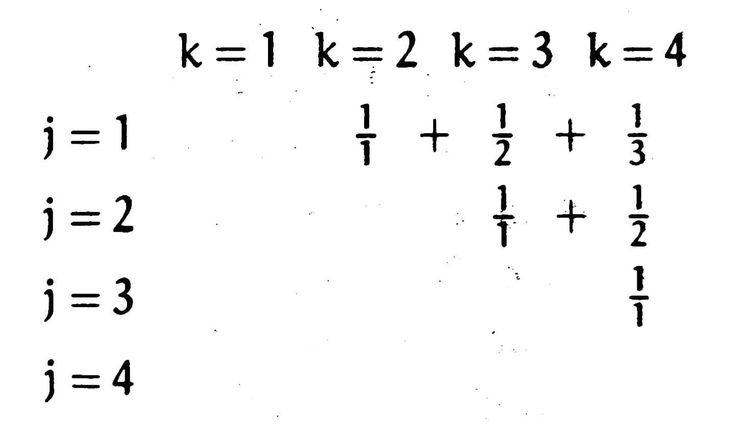
the left-hand side of the equation means for every $k$, sum up all items available in the $k$-th column, that is, all items in $J(k)$; the right-hand side is similar, $K^\prime(j)$ is the set of all items available in the $j$-th row.
2.5 General Methods
Method 0 is to look up. The authors suggested a few huge books for manual look ups. Fortunately, the on-line database OEIS is available; it is a more suitable tool than books for such knowledge.
Method 1 is guessing then proving. Since guessing needs flashes of inspiration, this method do not always work, and proving should in fact be a complement for other methods that establish sums from scratch.
Method 2 is the perturbation method. Perturb the sum a bit, then find relations between the perturbed sum and the original sum.
Method 3 is the repertoire method. This method still needs intuition to determine what form the recursion should be.
Method 4 uses infinite calculus to approximate the sum, then use other methods to compensate for the error terms.
Method 5 is to clever rewrite of the original sum. This method requires even more intuition than the repertoire method does. Expand a single sum to multiple sums to simplify the summand.
Method 6 is the topic of the next section.
Method 7 will be introduced in later chapters.
2.6 Finite and Infinite Calculus
Just like in calculus, we need a huge repertoire to evaluate sums effectively. Here are some useful formulas:
$$\begin{aligned}&x^{\underline{m+n}}=x^{\underline m}(x-m)^{\underline n};\\&\sum\nolimits_a^bc^x\delta x=\frac{c^b-c^a}{c-1};\\&\sum\nolimits_a^bx^{\underline m}\delta x=\begin{cases}\frac{x^{\underline{m+1}}}{m+1}\Big|_a^b,&\text{if $m\neq-1$;}\\H_x\Big|_a^b,&\text{if $m=-1$.}\end{cases}\end{aligned}$$
The relation of $\Delta(uv)=u\Delta v+{\rm E}v\Delta u$ yields the rule for summation by parts:
$$\sum u\Delta v=uv-\sum{\rm E}v\Delta u.$$
This rule is useful when $\sum{\rm E}v\Delta u$ is easier to evaluate than the original one.
2.7 Infinite Sums
In this section, we proved the validity of the three basic laws for absolutely convergent sums. Make sure the sum converges absolutely before applying these rules.